Understanding Muon

This post documents my current understanding of the Muon optimizer from my research. Much of Muon’s theoretical discussion remains scattered across blog posts, so I hope this makes its various design choices and versions easier to understand.

As a brief introduction, Muon is an optimizer designed for hidden layers of neural networks. Compared with the popular Adam/AdamW, Muon is particularly interesting because it is motivated by a clear theoretical objective rather than heuristic design choices. Muon has also surpassed AdamW in many benchmark settings, making it another go-to optimizer for large-scale training tasks.

I first derive the basic version of Muon , then walk through the rationales and derivations behind its different variants, and conclude with some further readings.

Basic Derivation

Let’s begin with notation. Let $\Weights$ denote the weight matrix, $\Gr$ the gradient matrix, $\Momentum$ the momentum-augmented gradient matrix, $\Orthogonal$ an orthogonalized matrix, $\eta$ the learning rate, and $\mu$ the momentum. I also use $\fanin$ and $\fanout$ throughout this post to denote a given layer’s fan-in and fan-out dimensions.

The following algorithm should look familiar if you have seen the Muon update rule before. Here, NS denotes the Newton-Schultz algorithm.

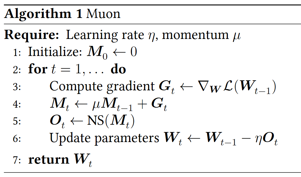
Let’s unpack how we arrive at the core update step:

\[\begin{equation} \Weights \gets \Weights - \eta \times \text{NS}(\grad[\Weights]\lossfunc) \label{eq:muon-update} \end{equation}\]

Our goal is to find a weight update that maximizes improvement in loss $\lossfunc$ while constraining the change in output ($\change y$) that we want to make in one step. In this case, we’ll use the spectral norm to measure the output change and write the problem as:

\[\begin{equation} \min_{\change \Weights} \langle \grad[\Weights]\lossfunc, \change \Weights \rangle _F \text{ subject to } \snorm{\change y} \le \eta \label{eq:output-constrained-objective} \end{equation}\]

The induced norm bound is:

\[\begin{equation} \snorm{\change y} = \snorm{\change \Weights x} \le \snorm{\change \Weights} \times \snorm{x} \label{eq:output-change-bound} \end{equation}\]

Using $\eqref{eq:output-change-bound}$, we can turn the constraint in $\eqref{eq:output-constrained-objective}$ into $\snorm{\change \Weights} \le \eta$, and the full problem becomes:

\[\begin{equation} \min_{\change \Weights} \langle \grad[\Weights]\lossfunc, \change \Weights \rangle _F \text{ subject to } \snorm{\change \Weights} \le \eta \label{eq:muon-objective} \end{equation}\]

See the appendix for a more in-depth derivation of $\eqref{eq:muon-objective}$ and the solution below, but to keep this section brief, we will jump to the solution. By performing an SVD on the gradient $\grad[\Weights]\lossfunc = U\Sigma V^\top$, we can solve the problem with:

\[\begin{equation} \change \Weights = -\eta \times UV^\top \label{eq:svd-optimal-update} \end{equation}\]

Using the Newton-Schultz algorithm to approximate the polar factor $UV^\top$ in $\eqref{eq:svd-optimal-update}$ without forming the SVD saves computational overhead and gives the core update rule in $\eqref{eq:muon-update}$.

Scale Factor Choice

Across different literature, you may encounter several versions of Muon. The three below are the most relevant here: the basic version above and the two variants provided by PyTorch. In PyTorch, pass “original” to the adjust_lr_fn parameter for the Keller Jordan version and “match_rms_adamw” for the Moonlight version.

\[\Weights[t] \gets \begin{cases} \Weights[t-1] - \eta \Orthogonal[t] & \textit{basic version} \\ \Weights[t-1] - \eta(\sqrt{\max(1, \frac{\fanout}{\fanin})}\Orthogonal[t] + \lambda \Weights[t-1]) & \textit{Keller Jordan Version} \\ \Weights[t-1] - \eta(0.2 \times \sqrt{\max(\fanout, \fanin)}\Orthogonal[t] + \lambda \Weights[t-1]) & \textit{Moonlight Version} \end{cases}\]

Keller Jordan Version

The Keller Jordan version above is the formulation used in the original Muon repository. Let’s first consider the $\frac{\fanout}{\fanin}$ component of the update. It is motivated by the $\mu$P line of work, which uses an RMS-to-RMS norm on the weight matrix instead of the spectral norm. This norm is defined as:

\[\begin{equation} \rmsrmsnorm{\Weights} := \max_{x \ne 0} \frac{\rmsnorm{\Weights x}}{\rmsnorm{x}} \label{eq:rms-to-rms-norm} \end{equation}\]

For this derivation, we make one key assumption: modern architectures usually normalize activations through LayerNorm or RMSNorm, which keeps hidden representations close to unit RMS magnitude. In math, this is:

\[\begin{equation} \rmsrmsnorm{x} \le 1 \end{equation}\]

The norm in $\eqref{eq:rms-to-rms-norm}$ helps make hyperparameters transferable across model width. You can read more about this in Tensor Programs V and the feature learning theory. Replacing the spectral norm with the RMS-to-RMS norm and using the preceding assumption gives:

\[\begin{equation} \rmsrmsnorm{\change \Weights} = \max_{x \ne 0} \frac{\rmsnorm{\change \Weights x}}{\rmsnorm{x}} = \sqrt{\frac{\fanin}{\fanout}} \snorm{\change \Weights} \label{eq:rms-spectral-relation} \end{equation}\]

Substituting $\eqref{eq:rms-spectral-relation}$ into $\eqref{eq:muon-objective}$ gives a new condition:

\[\begin{equation} \snorm{\change \Weights} \le \sqrt{\frac{\fanout}{\fanin}} \eta \label{eq:scaled-constraint} \end{equation}\]

Plugging $\eqref{eq:scaled-constraint}$ into the optimal solution gives the update rule:

\[\begin{equation} \Weights[t] \gets \Weights[t-1] - \eta\sqrt{\frac{\fanout}{\fanin}}\Orthogonal[t] \label{eq:keller-jordan-update} \end{equation}\]

This is as far as I have been able to make sense of this version of Muon. The clamp at $1$ in the Keller Jordan version clearly affects the update, but I have not found its exact motivation, so I leave it as an open question. I will return to weight decay in the discussion of the Moonlight version.

Moonlight Version

The Moonlight version above is commonly used because of its scalability and ease of tuning. Rather than tuning Muon’s hyperparameters from scratch, its $0.2\times \sqrt{\max(\fanout, \fanin)}$ factor allows a learning rate tuned for AdamW to be used directly with Muon. This factor is derived by matching Muon’s update RMS to AdamW’s.

The Muon is Scalable for LLM Training paper motivates this scale factor with two key facts. The first is the following lemma:

\[\begin{equation} \text{For a full-rank matrix parameter of shape} [A, B] \text{, its Muon update RMS is} \frac{1}{\sqrt{\max(A, B)}} \label{eq:moonlight-update-rms} \end{equation}\]

Second, AdamW has an update RMS of around $0.2$. By $\eqref{eq:moonlight-update-rms}$, multiplying the update by $0.2\times \sqrt{\max(\fanout, \fanin)}$ gives Muon approximately the same update RMS as AdamW. The paper empirically verifies that this makes the AdamW learning rate broadly transferable to Muon.

Finally, the paper addresses the addition of weight decay. It shows that Muon loses its advantage over AdamW in a larger model, while Muon with weight decay improves performance over both Muon and AdamW at that scale.

Additional Design Choices

Two additional choices are worth noting: Nesterov momentum and the orthogonalization method.

Momentum

Nesterov momentum is relatively straightforward. It empirically improves performance in many Muon training tasks, but it is often omitted for simplicity. PyTorch defaults to Nesterov momentum, though you can control it with the nesterov parameter.

Orthogonalization

For orthogonalization methods, all of the discussion above uses Newton-Schultz with 5 iterations. However, another popular method is the Polar Express algorithm with 5 iterations, which provides a more accurate approximation at a similar runtime. There’s also the more recent Cubic5 algorithm, an adaptive Newton-Schultz method that provides anywhere from 16–52% faster orthogonalization depending on the specific task tested.

An interesting aspect of orthogonalization in Muon is that the exact precision of the approximation does not seem especially beneficial for performance. Still, because Polar Express and Cubic5 have not yet been extensively tested, I would stick with the original Newton-Schultz algorithm for general use cases.

Sources

Bernstein, J. (2025). Deriving Muon. https://jeremybernste.in/writing/deriving-muon
Jordan, K., Jin, Y., Boza, V., You, J., Cesista, F., Newhouse, L., & Bernstein, J. (2024). Muon: An optimizer for hidden layers in neural networks. https://kellerjordan.github.io/posts/muon/
苏剑林. (2025). 为什么Adam的Update RMS是0.2？. https://kexue.fm/archives/11267
苏剑林. (2025). Muon优化器指南：快速上手与关键细节. https://kexue.fm/archives/11416
Liu, J., Su, J., Yao, X., Jiang, Z., Lai, G., Du, Y., Qin, Y., Xu, W., Lu, E., Yan, J., Chen, Y., Zheng, H., Liu, Y., Liu, S., Yin, B., He, W., Zhu, H., Wang, Y., Wang, J., … Yang, Z. (2025). Muon is Scalable for LLM Training. https://arxiv.org/abs/2502.16982
Amsel, N., Persson, D., Musco, C., & Gower, R. M. (2025). The Polar Express: Optimal Matrix Sign Methods and Their Application to the Muon Algorithm. https://arxiv.org/abs/2505.16932
Yang, G., Hu, E. J., Babuschkin, I., Sidor, S., Liu, X., Farhi, D., Ryder, N., Pachocki, J., Chen, W., & Gao, J. (2022). Tensor Programs V: Tuning Large Neural Networks via Zero-Shot Hyperparameter Transfer. https://arxiv.org/abs/2203.03466
Huang, H. (2026). How Much Orthogonalization Does Muon Need? https://arxiv.org/abs/2606.00371
Chollet, F., & others. (2015). Keras. https://keras.io.
Bernstein, J., & Newhouse, L. (2024). Modular Duality in Deep Learning. https://arxiv.org/abs/2410.21265
Pethick, T., Xie, W., Antonakopoulos, K., Zhu, Z., Silveti-Falls, A., & Cevher, V. (2025). Training Deep Learning Models with Norm-Constrained LMOs. https://arxiv.org/abs/2502.07529

Appendix

Muon Derivation

Let’s first expand on how we obtained the problem. For a small parameter update from the update step, we can use the first-order Taylor expansion to approximate the change in loss:

\[\begin{equation} \lossfunc(\Weights + \change\Weights) \approx \lossfunc(\Weights) + \langle \grad[\Weights]\lossfunc, \change \Weights \rangle _F \label{eq:first-order-taylor} \end{equation}\]

By $\eqref{eq:first-order-taylor}$, decreasing the loss means minimizing $\langle \grad[\Weights]\lossfunc, \change \Weights \rangle _F$, which gives the objective in $\eqref{eq:muon-objective}$.

Now, to solve $\eqref{eq:muon-objective}$, let $\grad[\Weights]\lossfunc = U\Sigma V^\top$ be its SVD. We get:

\[\begin{align} \langle \grad[\Weights]\lossfunc, \change \Weights \rangle _F &= \trace(\grad[\Weights]\lossfunc^\top \change\Weights) \label{eq:objective-trace} \\ &= \trace(V\Sigma U^\top \change\Weights) \notag \\ &= \trace(\Sigma U^\top \change\Weights V) \label{eq:objective-svd-trace} \end{align}\]

Let $Z := U^\top \change\Weights V$. Since $\Sigma = diag(\sigma_1, \dots, \sigma_r)$, $\eqref{eq:objective-svd-trace}$ reduces further to:

\[\begin{equation} \trace(\Sigma U^\top \change\Weights V) = \trace(\Sigma Z) = \sum_{i=1}^{r} \sigma_i Z_{ii} \label{eq:objective-diagonal} \end{equation}\]

Since multiplying by orthogonal matrices can’t increase the spectral norm, and $U$ and $V$ are both orthogonal matrices, we have:

\[\begin{equation} \snorm{Z} = \snorm{ U^\top \change\Weights V } \le \snorm{\change\Weights} \label{eq:orthogonal-spectral-bound} \end{equation}\]

Using the constraint in $\eqref{eq:muon-objective}$ and $\eqref{eq:orthogonal-spectral-bound}$, we know $\snorm{Z} \le \eta$. In particular, $Z_{ii} \ge -\eta$ for all $i$.

Since every $\sigma_i \ge 0$, $\eqref{eq:objective-diagonal}$ gives the following lower bound on the objective:

\[\begin{equation} \langle \grad[\Weights]\lossfunc, \change \Weights \rangle _F \ge -\eta \sum_{i=1}^{r} \sigma_i \label{eq:objective-lower-bound} \end{equation}\]

Now observe that choosing $\change \Weights = -\eta UV^\top$ attains the lower bound in $\eqref{eq:objective-lower-bound}$:

\[\begin{align} \langle \grad[\Weights]\lossfunc, -\eta UV^\top \rangle _F &= -\eta \trace((U\Sigma V^\top)^\top UV^\top) \notag \\ &= -\eta \trace(V\Sigma U^\top UV^\top) \notag \\ &= -\eta \trace(V\Sigma V^\top) \notag \\ &= -\eta \trace(\Sigma) \notag \\ &= -\eta \sum_{i=1}^{r} \sigma_i \label{eq:objective-attained} \end{align}\]

Thus, $\eqref{eq:objective-attained}$ shows that $\change \Weights = -\eta UV^\top$ is the optimal update in $\eqref{eq:svd-optimal-update}$.

Finally, to avoid the computationally expensive orthogonalization computation in $\eqref{eq:svd-optimal-update}$, we use the Newton-Schultz algorithm to approximate this calculation, which gives the final update step in $\eqref{eq:muon-update}$.